Welcome to the QUBES Hub BIOSC0160 students

You have landed in the right place for the Community Dynamics Recitation

We are going to be using the NetLogo software today but you won't need to download anything. We will run it remotely (on servers located elsewhere) through your web browser.

To do this you will first need to create a user account by clicking the "Login" button and linking your Google account (see picture).



When you have successfully created an account you will be placed in your "Dashboard". Use the back button or follow this link again http://bit.ly/communitydynamics to return to the exercise.

Community Population Dynamics Recitation

This week we will use a simple model of a food chain to extend our models of individual populations and explore how populations interact with one another within a community. The model we will use this week is modified from:

Wilensky, U. & Reisman, K. (2006). Thinking like a Wolf, a Sheep or a Firefly: Learning Biology through Constructing and Testing Computational Theories -- an Embodied Modeling Approach. Cognition & Instruction, 24(2), pp. 171-209.

We will be modeling trophic interactions using an agent-based modeling environment called NetLogo. In agent-based models simple rules describe the actions of different objects in the model and we can study the patterns of behaviors that emerge. We will model:

• A Primary Producer – Grass; it grows; we can adjust how quickly it regrows after being eaten.
• A Primary Consumer – Sheep; they move around and eat grass, reproduce, and die; we can control their initial population size, digestive efficiency, and reproductive rate.

• A Secondary Consumer – Wolf; they move around, eat sheep, reproduce, and die; we can control their initial population size, digestive efficiency, and reproductive rate. 

Manipulating the Software

There are only a few parameters that can be set but there are a wide range of questions we can ask and patterns we can observe.

• Use the SETUP button to populate the environment. 
• Press the GO button to start and stop the simulation.
• The output is displayed in both the number and positions of organisms in the map and as population sizes over time in the graph.
• You can adjust the sliders to change the variables.
• You can reset the simulation by stopping it and then clicking SETUP.
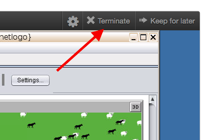
• When you are done (or you need to reset to the original settings) click TERMINATE

Activity 1: Orienting to the Model

1. Open THIS VERSION of the model.
   NOTE: In this set-up we have the grass “turned off” meaning that the sheep can have all the energy they need and they do not impact the grass population.
2. Press “SETUP” to initiate the simulation and then press “GO” to start it.
3. Stop the simulation when one of the species goes locally extinct.
4. Qualitatively describe what happened in your trial?
5. Quantitatively describe what happened in your trial? (moving the cursor over the graph will give you values)
   1. When did the sheep population peak and how large was their population?
   2. When did the wolf population peak and how large was their population?
   3. Who when extinct and when?
6. Press “SETUP” to reset the simulation and run it again.
7. Did you get the same qualitative results? Quantitative results?
8. Check with your neighbors and see if they got a different result.

Be prepared to use the following ideas to discuss your modeling:

• Population growth / population shrinkage
• Exponential growth phase / Logistic growth phase
• Carrying capacity
• The relative timing of each population’s growth and decline
• Relative population sizes (this will show up better in the next model)
• Stability of the community
• Behavior of stochastic models

Activity 2: Using a 3-Species model

1. Turn on the grass so that the primary producer population can change.
2. Run your model for around 1000 time steps.
3. Do you see patterns in:
   1. The relative timing of each population’s growth and decline
   2. Relative population sizes
   3. Stability of the community
4. Repeat the trial and run the model for longer time periods – are the cycles stable? Do the populations go through about the same range of sizes at about the same intervals?

Activity 3: "What if …" Modeling Questions

Now that we have the mechanics and basic behaviors sorted out let’s do some exploration. Choose one or two of the following questions and investigate them using this community model.

1. How sensitive is the model to the starting population sizes of the predator and prey? Is it population size per se that is important or is it relative population size between predator and prey that matters?
2. Model the introduction of a species into a habitat where it doesn’t face the normal constraints on population growth – for a while anyways (e.g., St. Matthew Island reindeer). Describe the pattern of population growth (and shrinkage) that you see. Set wolves to 0 - there were no predators on St. Matthew; set the initial sheep number to a low value - they only dropped off a few caribou; set the grass regrowth time as very slow - it was primarily lichen which grows very slowly; and double the sheep reproductive rate to 8% - less time worrying about food and predators = more time reproducing. 
3. Explore the impact of varying one of the other sheep or wolf parameters (digestive efficiency or reproductive rate). You can change these after the community has been cycling for a while by pausing the simulation, changing the variable and then pressing GO again. Predict how your change will impact the population dynamics and then test your predictions with several trials.
4. Can you figure out ways to model these biological scenarios?
   1. A long term drought that reduces plant growth.
   2. Introduce a parasite that interferes with the wolf’s energy gain from food.
   3. Change the food source for sheep so it is more nutritious.
   4. Introduce a different species of wolf that has a higher reproductive rate.

Post Recitation Activities –

The post recitation is available on Mastering Biology.